Comparison of Four-Dimensional Flow Magnetic Resonance Imaging and Particle Image Velocimetry to Quantify Velocity and Turbulence Parameters

Abstract

Although recent advances of four-dimensional (4D) flow magnetic resonance imaging (MRI) has introduced a new way to measure Reynolds stress tensor (RST) in turbulent flows, its measurement accuracy and possible bias have remained to be revealed. The purpose of this study was to compare the turbulent flow measurement of 4D flow MRI and particle image velocimetry (PIV) in terms of velocity and turbulence quantification. Two difference flow rates of 10 and 20 L/min through a 50% stenosis were measured with both PIV and 4D flow MRI. Not only velocity through the stenosis but also the turbulence parameters such as turbulence kinetic energy and turbulence production were quantitatively compared. Results shows that 4D flow MRI velocity measurement well agreed with the that of PIV, showing the linear regression slopes of two methods are 0.94 and 0.89, respectively. Although turbulence mapping of 4D flow MRI was qualitatively agreed with that of PIV, the quantitative comparison shows that the 4D flow MRI overestimates RST showing the linear regression slopes of 1.44 and 1.66, respectively. In this study, we demonstrate that the 4D flow MRI visualize and quantify not only flow velocity and also turbulence tensor. However, further optimization of 4D flow MRI for better accuracy might be remained.

1. Introduction

Turbulence in blood flow is known to create irregular fluid motion and chaotic changes in pressure and velocity. While blood flow mostly exists as laminar flow state, high flow rate through the heart valve or pulsatility of aortic flow locally develop turbulent blood flow. Local vascular obstructions due to atherosclerosis and a stenotic heart valve are widely known pathophysiological conditions developing turbulent blood flow [1].

Turbulent blood flows in humans and animals have been postulated to contribute to a variety of pathological conditions. Turbulent flow is associated with high oscillatory shear stresses which can damage the endothelial layer and red blood cells [2,3]. A malfunction of the endothelial layer is associated with the initial development and progress of atherosclerosis and aortic dilatation [4,5]. The abnormal level of turbulence in the blood flow has been considered as a fluid-dynamic biomarker for early diagnosis of vascular diseases.

Despite of its clinical significance, turbulence measurement in the blood flow has been rare due to the lack of the measurement technique. A constant temperature hot-film anemometer was previously utilized to analyze the fluctuating velocities associated with turbulent flow [6]. However, the invasive measurements have been restricted owing to ethical issues. Instead, many experiments have been conducted with non-invasive methods, computational fluid dynamic (CFD), and imaging modalities such as echocardiography and magnetic resonance imaging (MRI) [7,8].

Recently, time-resolved, three-directional, and three-dimensional phase-contrast magnetic resonance imaging (commonly known as 4D PC-MRI or 4D flow MRI) has been widely used to measure complicated blood flows. The conventional 4D flow MRI technique measures spatiotemporally averaged velocities within each voxel, meaning the resultant voxel velocity is insensitive to turbulent flow effects. Recently, this technique was extended to estimate the turbulent intensity of small-scale velocity fluctuations in cardiovascular flows. A previous study confirmed the feasibility of turbulent kinetic energy (TKE) estimation at clinically practical spatial resolutions [9]. This 4D flow MRI turbulence mapping technique was further generalized with a six-directional icosahedral (ICOSA6) flow-encoding scheme, rather than the conventional four-point (4P) flow-encoding scheme. The generalized technique was successfully applied to measure all components of the Reynolds stress tensor (RST) in turbulent flows and used for quantifying hemodynamic abnormality in the blood flow.

Despite numerous validations on the velocity measurement of the 4D flow MRI, accuracy and uncertainty of the 4D flow MRI for the turbulence quantification has rarely been investigated. Petter et al. validated the turbulence intensity of the 4D flow MRI with a laser Doppler anemometer (LDA) [10]. Ha et al. validated the TKE quantification of the 4D flow MRI by comparing TKE through the stenosis with particle image velocimetry (PIV) [9]. Although previous studies on ICOSA6 4D flow MRI have highlighted its clinical potential of the quantification of full Reynolds stress for hemodynamic blood damage prediction and irreversible pressure loss estimation [11]; however, the questions related to its measurement uncertainty/accuracy and possible bias have not yet been well scrutinized. In particular, the off-diagonal portions of the Reynolds stress have rarely been validated.

The PIV has been widely used as a gold-standard technique for validating the flow analysis in numerous biomedical applications. The PIV directly captures the optical image of the seeding particle and estimates flow velocities based on particle displacement. Previously, complicated blood flows through biomedical devices such as left ventricular assist devices were simulated with CFD and the results were validated with experimental measurements with PIV [12,13]. Additionally, the PIV has been widely used to validate the 4D flow MRI measurement of velocity and turbulence in a stenosed phantom [9,14].

The purpose of this study was to compare the 4D flow MRI and PIV methods for velocity and turbulence measurements. In this study, we measured the steady flow through the stenosis at two different flow rates (10 and 20 L/min). The velocity and turbulence parameters including TKE and turbulence production (TP) measured from the 4D flow MRI and conventional PIV methods were quantitatively investigated. This effort will provide the validation of the 4D flow MRI for quantification of turbulence parameters.

2. Materials and Methods

2.1. Experimental Setup

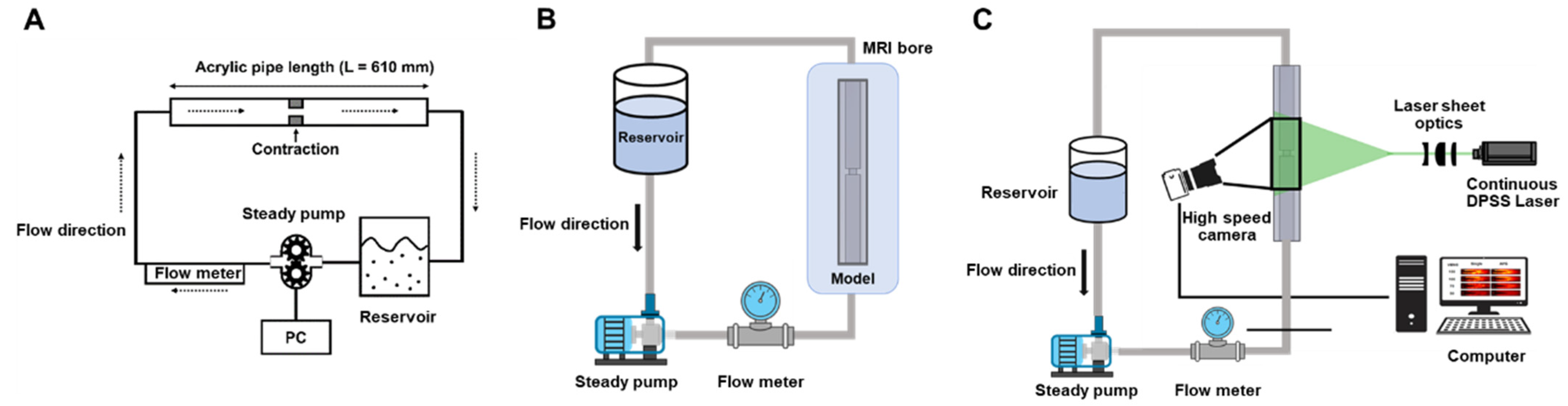
Experimental measurements were conducted using the 4D flow MRI on an in-vitro flow phantom under various scan conditions to analyze the robustness of ICOSA6 for turbulence quantification. The rectangular flow phantom used for this experiment was a sudden contraction/expansion model with a 75% reduction in area (50% in length, Figure 1). The upstream size without any constriction was 25 mm. To stabilize the upstream flow in the constriction region, a 0.3 m straight section was used. Another 0.3 m straight section was placed downstream from the constriction.

The working fluids were water and a blood analog composed of a 40:60 glycerol/water mixture (by mass). The density and dynamic viscosity of the working fluid were 1053.8 kg/m³ and 3.72 × 10⁻³ kg/m⋅s, respectively. The working fluid was circulated through the flow circuit system at a constant flow rate using a centrifugal pump (EHEIM Universal 3400, Deizisau, Germany). Flow rates of 10 and 20 L/min were set by monitoring with an electromagnetic flowmeter (VN20, Wintech Process, Seoul, Korea). The corresponding Reynolds numbers of the inlet flow at 10 and 20 L/min were 1888 and 3777, respectively. The temperature of the fluid during experimentation was 20 °C. A contrast agent, 30 mL of contrast agent (0.5 mmol/kg, gadofosveset trisodium, VasovistVR, Bayer Schering Pharma AG, Berlin, Germany) was added to 40 L of the working fluid for MRI measurement.

2.2. 4D Flow MRI Measurement

The 4D flow MRI measurements were conducted using a clinical 1.5T MRI scanner (1.5T Philips Achieva, Philips Medical Systems, Best, The Netherlands). The ICOSA6 method modifies the conventional four-point 4D flow MRI to employ a six-directional icosahedral flow encoding and one flow-compensated reference encoding. Velocity-encoding (Venc) parameter values from 100 to 150 cm/s were used for the turbulence quantification while the Venc of 450 cm/s was used for the velocity measurement. The echo time (TE) and temporal resolution ranges were 2.5–3.0 ms and 3.4–4.4 ms, respectively. The flip angle was 10°. The matrix size range was 128  ×  128 ×  24 voxels with a 2.0 mm isotropic voxel size. Partial echo with a factor of 0.725 along the frequency-encoding directions was used to minimize TE. An artificial electrocardiogram with an interval of 1000 ms was used to measure and reconstruct multiple phases of the steady flow.

2.3. 4D Flow MRI Turbulence Quantification

For the conventional 4D flow MRI, the MRI signal S(k_v) for a velocity distribution s(v) is expressed by a Fourier transformation as

$$S\left(k_v\right)=C{{\displaystyle \int }}_{-\infty }^{\infty }s\left(v\right)e^{-{ik}_{v}v}dv$$

(1)

where C is a constant scaling factor influenced by the relaxation parameter, spin density, receiver gain, etc. k_v represents the level of flow sensitivity, which is related to Venc as k_v = π/Venc. When turbulent flow occurs in the region of interest, the intravoxel velocity variance (IVVV) of the turbulent flow along the i direction, denoted by ${\sigma }_i^2$, can be estimated from the magnitude ratio between the reference signal without velocity encoding S(0) and the signal with velocity encoding along the i direction S_i(k_v) as

$${\sigma }_i^2=\overline{u_i^{\prime }{u}_i^{\prime }}=\frac{2}{k_v^2}\ln \left(\frac{\left|S_i\left(0\right)\right|}{\left|S_i\left(k_v\right)\right|}\right)\left(m^2/s^2\right)$$

(2)

Here, $u_i^{\prime }$ denotes the fluctuating portion of the velocity and the $\overline{ }$ symbol indicates an averaging operation.

When non-orthogonal flow encodings are distributed in a three-dimensional Cartesian space, the obtained velocity and IVVV values can be decomposed into orthogonal components and covariance terms. Therefore, three velocity components (u, v, and w) and the Reynolds stress component tensor R_ij can be obtained by measuring six non-orthogonal velocity encodings and finding the least-square solutions of the six-directional phase and magnitude data. R_ij is a six-element symmetric tensor defined as [11]

$$R= \rho \left[\begin{array}{ccc}\overline{u_1^{\prime }{u}_1^{\prime }}& \overline{u_1^{\prime }{u}_2^{\prime }}& \overline{u_1^{\prime }{u}_3^{\prime }}\\ \overline{u_2^{\prime }{u}_1^{\prime }}& \overline{u_2^{\prime }{u}_2^{\prime }}& \overline{u_2^{\prime }{u}_3^{\prime }}\\ \overline{u_3^{\prime }{u}_1^{\prime }}& \overline{u_3^{\prime }{u}_2^{\prime }}& \overline{u_3^{\prime }{u}_3^{\prime }}\end{array}\right]$$

(3)

Based on the velocity and Reynolds stress values obtained from the ICOSA6 sequence, the TKE of the flow can be calculated from the IVVV in each direction as

$$TKE=\frac{1}{2}\rho \left(\overline{u_1^{\prime }{u}_1^{\prime }}+\overline{u_2^{\prime }{u}_2^{\prime }}+\overline{u_3^{\prime }{u}_3^{\prime }}\right)\left(\mathrm{J}/{\mathrm{m}}^3\right)$$

(4)

where $\rho$ is the fluid density. Turbulent production (TP) can be calculated directly as

$$TP=-R_{ij}{S}_{ij}\left(\mathrm{J}/\mathrm{kg}·\mathrm{s}\right)$$

(5)

where S_ij represents the strain rate tensors of the mean velocity field. To compare the 4D flow MRI measurement with the two-dimensional PIV data, the velocity fluctuation is assumed to be two dimensional and the slice-directional velocity was neglected throughout this study.

2.4. Post-Processing of 4D Flow MRI Data

All raw data were exported from the scanner using the Pack’n Go tool (Gyrotool LLC, Zurich, Switzerland) and reconstructed using an offline reconstruction tool (ReconFrame, Gyrotool LLC, Zurich, Switzerland). Custom MATLAB code was used for the reconstruction of velocity and Reynolds stress values from the icosahedral flow encoding, as described in previous works [15,16]. To extract the flow velocity, the acquired data with the highest Venc values (450 cm/s) were used. To correct background offset, the velocity field obtained without any flow was used to correct the velocity offsets caused by background phase errors following the reference [11].

2.5. Setup of PIV

The PIV experimental setup consists of a high-speed camera, laser, seeding particle, and experimental model. The particles used in the experiment are hollow glass spheres (HGS), with diameters in the range of 2–20 μm, density = 1.1 g/cm³. The flow field was illuminated with a 0.5-mm-thick thin laser sheet using 532 nm continuous DPSS Laser (Changchun New Industries Optoelectronics Co., Ltd., Changchun, Jilin, China). A high-speed camera (4000 fps, 1280 × 512; VEO 710L, Vision Research lnc., Wanye, NJ, USA) is positioned perpendicular to the flow to measure velocity fields at the center plane of the model. The resolution of the camera was 0.54 $\mathsf{\mu }\mathrm{m}$/pixel with particle sizes of 2–4 pixels in the image. The measurements were taken at three location sections: stenosis apex, upstream, and downstream of the stenosis. These measurement data were combined at the post-processing.

2.6. PIV Analysis

The PIV analysis was performed using PIVlab built on the MATLAB platform (MathWorks, Natick, MA, USA). At each measurement plane, 19,000 image pairs were used for vector field calculation. A multi-grid interrogation scheme was adopted using 64 × 64 and 32 × 32 of interrogation windows with 50% overlapping. A fast Fourier transform (FFT)-based cross-correlation PIV algorithm was applied. The distance between two adjacent velocity vectors was 16 pixels, which corresponds to 0.09 mm. The results were resampled with bilinear interpolation to match the resolution and field of view of the PIV data with the 4D flow MRI velocity data.

The obtained velocity fields were statistically analyzed to obtain their mean and fluctuation components. Each instantaneous velocity vector u(t) in steady flow can be decomposed into a time-averaged mean velocity component and fluctuating velocity component u′(t)

$$\overline{u}=\frac{1}{N}{\displaystyle \sum }_{t=1}^{N}u{\left(t\right)}_{ },u\left(t\right)=\overline{u}+u^{\prime }\left(t\right)$$

(6)

where N is the number of velocity frames. The TKE and TP were estimated from Equations (3) and (5) using Equation (6).

2.7. Statistics

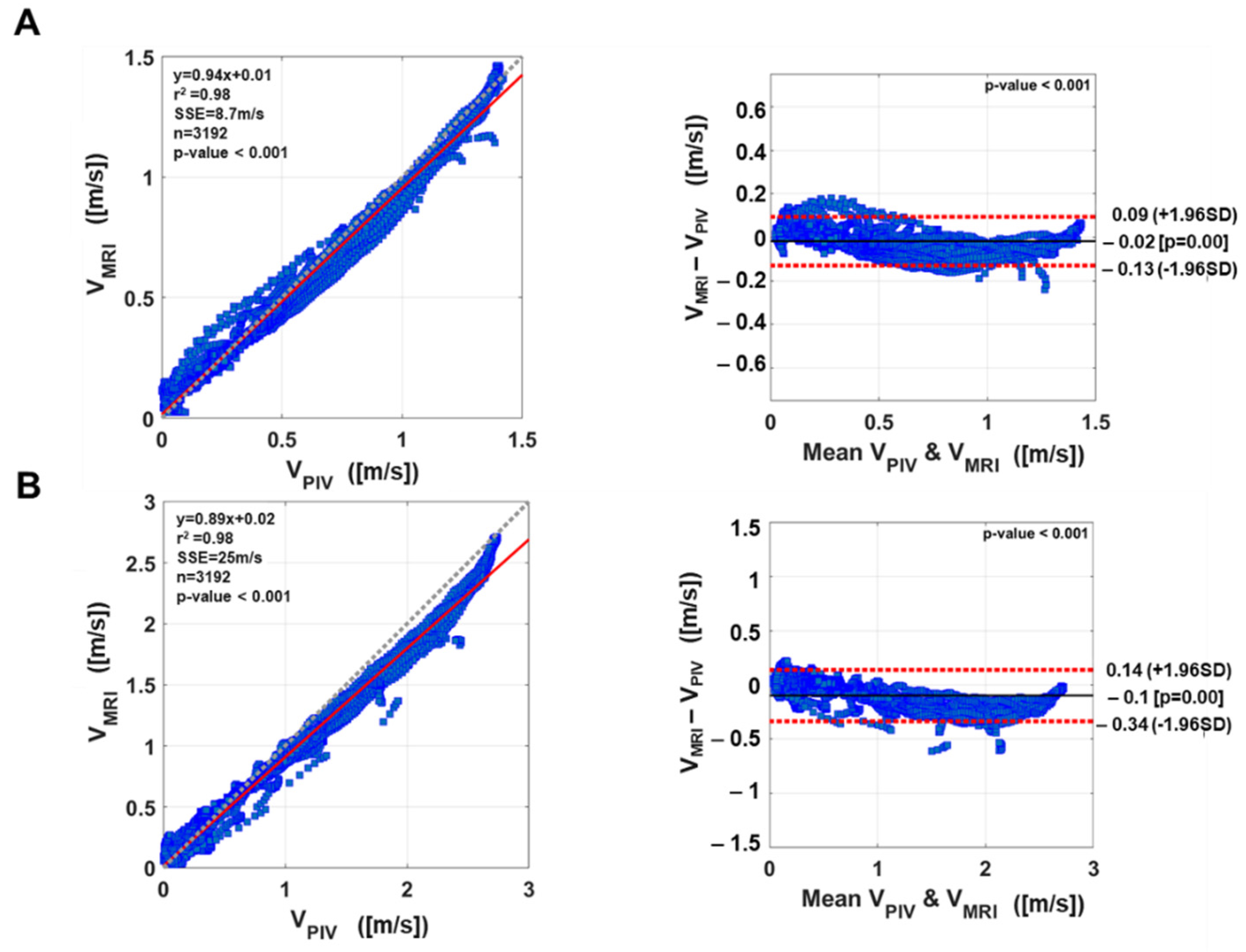
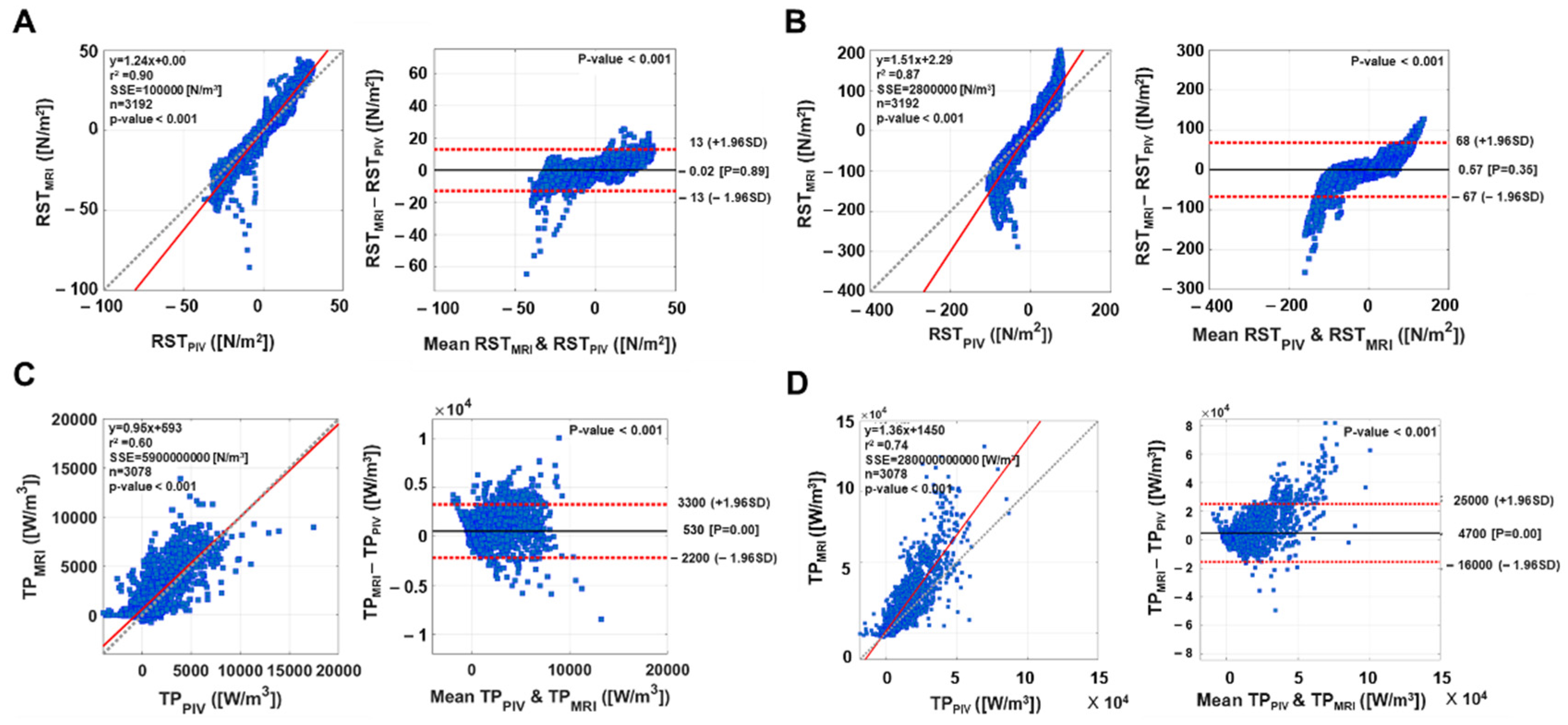
The Bland–Altman analysis evaluated the linear regression and an agreement interval of the 4D flow MRI and PIV measurements. The slope of the linear regression mean bias and 95% agreement interval were analyzed. Solid and dotted lines in the Bland–Altman plot indicate the mean difference and 1.96 standard deviation (SD) with a 95% limit of agreement. Plane and total turbulent values indicate mean ± standard error (SE).

3. Results

3.1. Velocity Comparison

The mean velocity measurements from the 4D flow MRI and PIV are qualitatively well agreed. Peak velocity at the stenosis apex was 1.47 m/s and 1.43 m/s at Q = 10 L/min, 2.87 m/s and 2.84 m/s at Q = 20 L/min. At the post-stenosis, the 4D flow MRI was slightly underestimated where the turbulent flow develops (Figure 2). The slope of linear regression was 0.94 with r² = 0.98 and 0.89 with r² = 0.98 at the flow rates of 10 and 20 L/min, respectively (Figure 3). The mean bias with 95% limits of agreement was −0.02 ± 0.11 m/s and 0.10 ± 0.24 m/s at the flow rates of 10 and 20 L/min, respectively.

3.2. TKE Comparison

The TKE estimation from the 4D flow MRI and PIV showed that both measurements are qualitatively agreed. Both measurements clearly showed the development of turbulence at the stenosis and post-stenosis along the boundary layer of the jet flow (Figure 4). The largest TKE at X/D ≈ 4 and the elevation of the TKE at the larger flow rate were observed in both measurements. Compared to the PIV measurement, the 4D flow MRI shows overall overestimation in the TKE field. The peak TKE of the 4D flow MRI was approximately 1.5 folds larger than that of PIV. The overestimation of the 4D flow MRI was shown regardless of the flow rate. The slope of linear regression was 1.44 with r² = 0.68 and 1.66 with r² = 0.78 at the flow rates of 10 and 20 L/min, respectively (Figure 5). The mean bias with 95% limits of agreement was 13.9 ± 34.2 J/m³ and 59.3 ± 111.3 J/m³ at the flow rates of 10 and 20 L/min, respectively. The TKEplane, which is the cross-sectional sum of TKE at each plane. Consequently, a total TKE of the 4D flow MRI and PIV was 3.8 ± 0.3 mJ and 2.2 ± 0.0 mJ, 13.2 ± 1.1 mJ and 8.7 ± 0.0 mJ at 10 and 20 L/min, respectively (Figure 6).

3.3. Reynolds Stress Tensor (RST) and TP Comparison

One off-diagonal element $\overline{u^{\prime }{v}^{\prime }}$ among six element RST was shown for clarity (Figure 7). The $\overline{u^{\prime }{v}^{\prime }}$ component from the 4D flow MRI and PIV showed as qualitatively similar but locally different. Both measurements clearly showed the development of RST at the stenosis and post-stenosis along the boundary layer of the jet flow (Figure 7).

An erroneous component was observed at X/D < 0 from both measurements. At the post-stenosis for X/D > 0, the 4D flow MRI overall overestimated RST with slopes of the regression line of 1.24 and 1.51 with r² = 0.90 and r² = 0.87 at the flow rates of 10 and 20 L/min, respectively. The mean bias with 95% limits of agreement was −0.0 ± 12.9 N/m² and 0.6 ± 67.6 N/m² at the flow rates of 10 and 20 L/min, respectively (Figure 8).

The TP indicated that the slope of linear regression line was 0.95 with r² = 0.60 and 1.67 with r² = 0.78, respectively. The mean bias with 95% limits of agreement was 525.6 ± 2726.5 W/m³ and 4924.1 ± 21,857.5 W/m³ at the flow rates of 10 and 20 L/min, respectively.

A total TP of the 4D flow MRI and PIV was 118.8 ± 27.8 mW and 99.0 ± 15.7 mW at 10 L/min, 891.3 ± 189 mW and 621.8 ± 71.9 mW at 20 L/min. The extent of overestimation and measurements uncertainty of the total TP was significantly larger at 20 L/min compared to 10 L/min (Figure 9).

3.4. 4D Flow MRI Measurement at the Pulsatile Flow Condition

The measurement showed that 4D Flow MRI clearly can visualize the development of turbulent flow during the pulsation. The velocity, TKE, and TP estimations of the 4D flow MRI were successfully mapped for the pulsatile flow conditions (Figure 10). While the instantaneous flow rate is greatest with 14.2 L/min at approximately 0.23 s, the velocity and turbulent parameters also have peak values. The measurement shows that the choice of Venc affects the SNR of the turbulence flow measurement. When the Venc was 100 cm/s, velocity, TKE, and TP were measured with high signal-to-noise ratio (SNR), and each peak value was 2.28 m/s, 601.8 J/m³, and 64.9 mW/m³. When the larger Venc was used, the sensitivity of the total TP and TKE were reduced but the results showed the same trend of turbulence (Figures S1–S3 in the Supplementary Materials).

4. Discussion

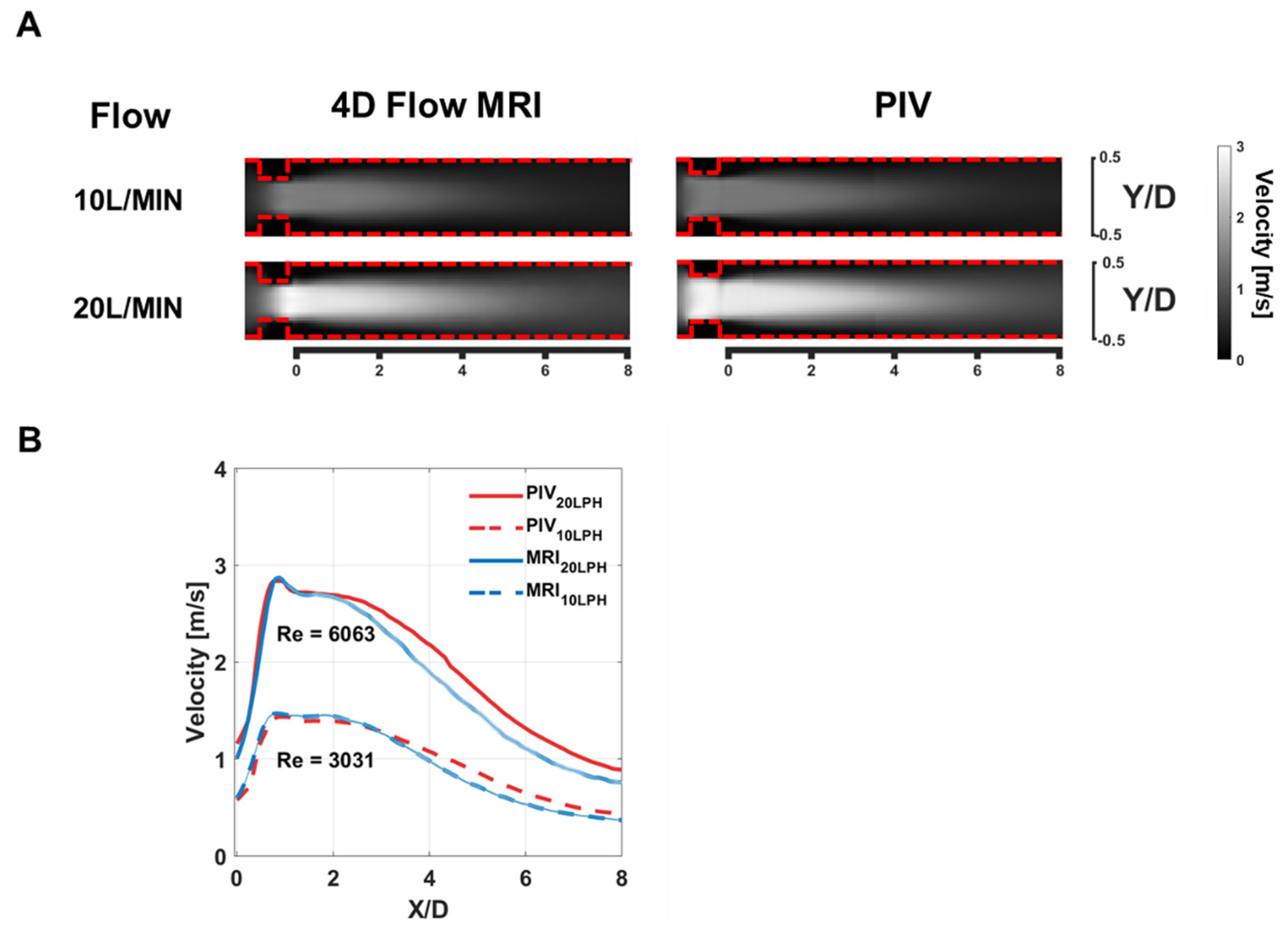
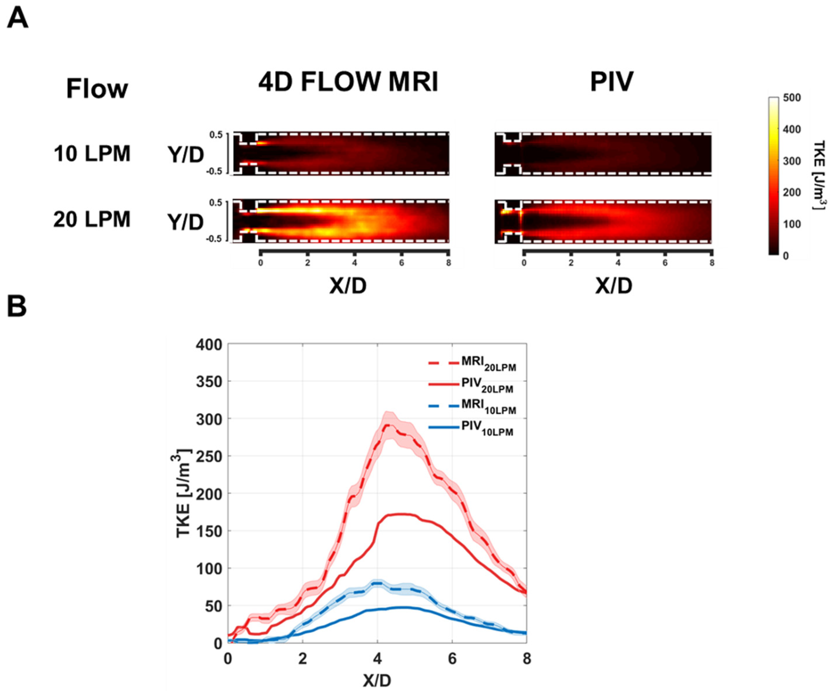
The purpose of this study was to validate the 4D flow MRI velocity and turbulence measurements against PIV measurements. The key findings of the study are that (i) the velocity measurements from the 4D flow MRI and PIV were qualitatively well agreed while the 4D flow MRI slightly underestimated the velocity at the post-stenotic turbulent flow region. (ii) TKE measurements from the 4D flow MRI and PIV were linearly correlated, but the 4D flow MRI shows overall overestimation in the TKE field. (iii) 4D flow MRI has potential to visualize not only diagonal but also off-diagonal elements of the RST, despite relative overestimation compared to those of PIV.

Despite good agreement in the peak velocity measurement, the 4D flow MRI showed underestimation at the post-stenosis flow region. Previous studies have investigated the accuracy of the 4D flow MRI velocity measurements. An earlier study compared the stenotic flow velocity with a low level of turbulence (Re < 550) from the 4D flow MRI and PIV. Results demonstrated that both measurements were linearly correlated for both steady and pulsatile flow conditions [17]. More recently, the comparison between the 4D flow MRI and CFD showed that the peak velocity and post-stenosis velocity of the 4D flow MRI are significantly underestimated depending on the spatial resolution [18]. Another validation study on the flow through an in-vitro aortic valve also showed that a high level of turbulence can lead to a measurement bias due to inaccurate forward and backward flow quantification [19]. The present study showed that although the 4D flow MRI gives accurate peak velocity, the velocity at the post-stenotic region is significantly underestimated. This indicates that the flow rate quantification downstream of the heart valve may induce a flow rate underestimation. If possible, the flow quantification upstream of the valve could be a better option because the turbulence level should be significantly lower upstream of the valve.

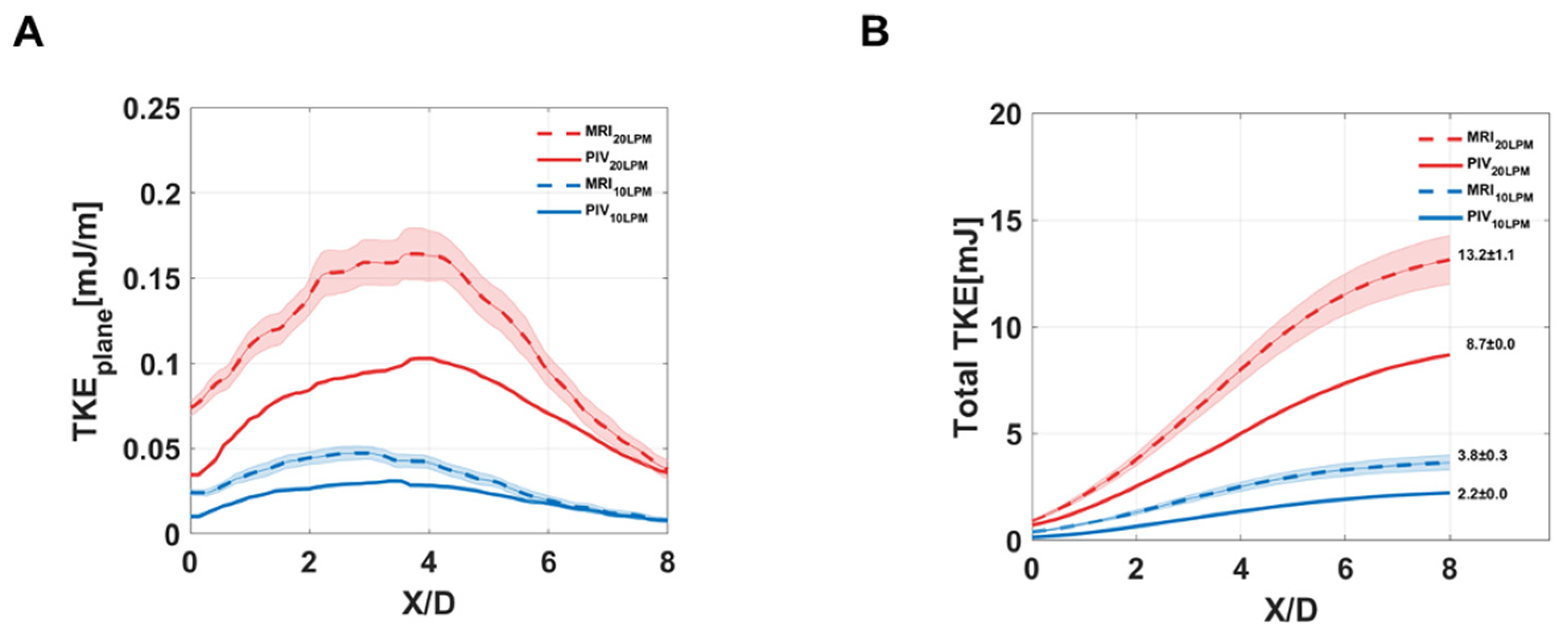
The present study showed that TKE estimations from the 4D flow MRI and PIV are linearly correlated despite the magnitude of TKE was overestimated in the 4D flow MRI.

The current 4D flow MRI turbulence estimation is based on intravoxel mean velocity distribution. Therefore, the mean velocity variation along the boundary layer of the jet flow can affect the results. Previously, it has been reported that MRI turbulence quantification is overestimated owing to the joint intravoxel velocity distribution that is obtained by convolution of the turbulence velocity distribution and the mean velocity variation [20]. The extended TKE estimation to compensate the mean velocity variation effect was also proposed, however, the experimental demonstration has not been performed mostly because of the increased number of MRI scans and correspondingly increased scan time.

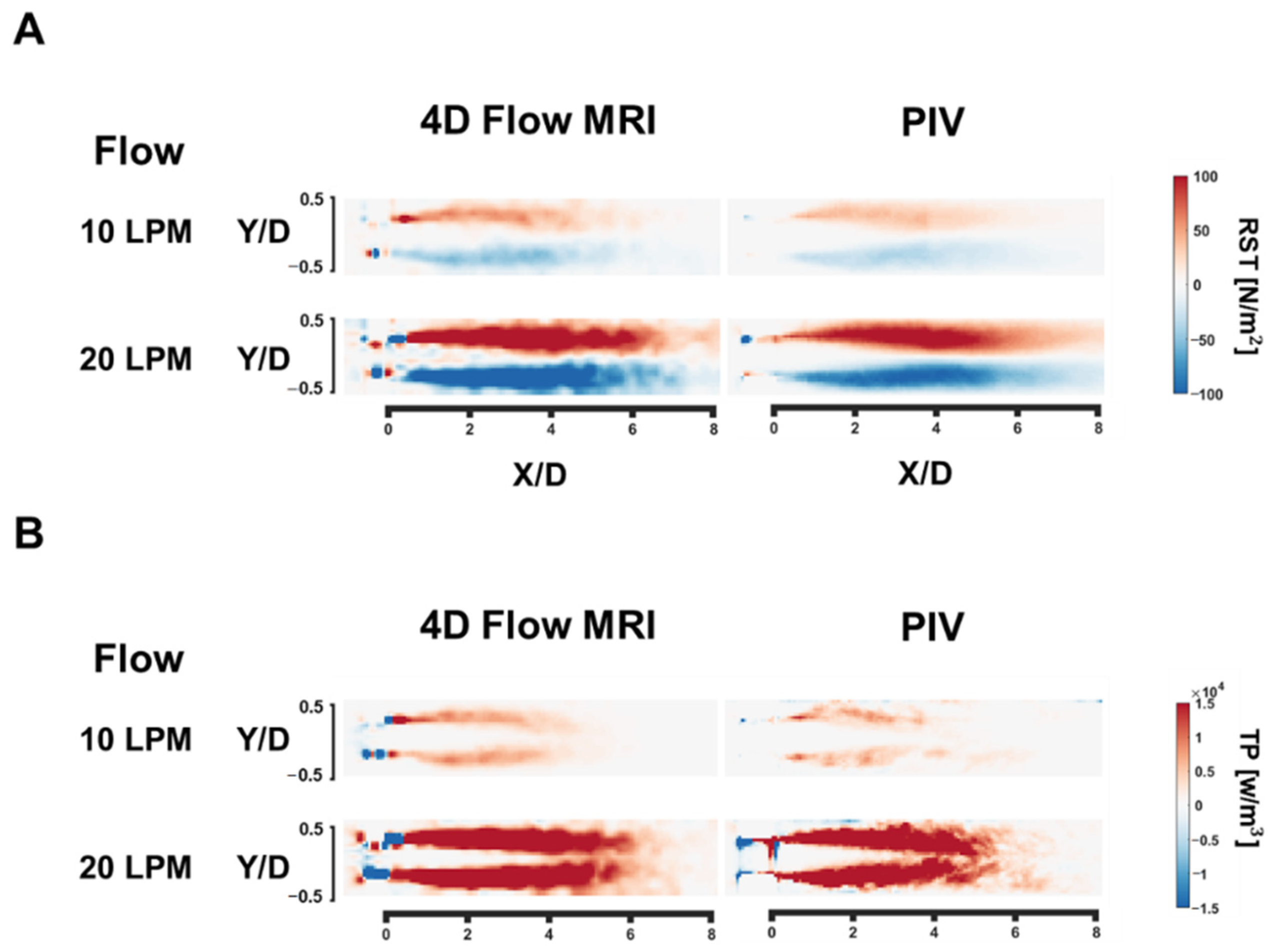
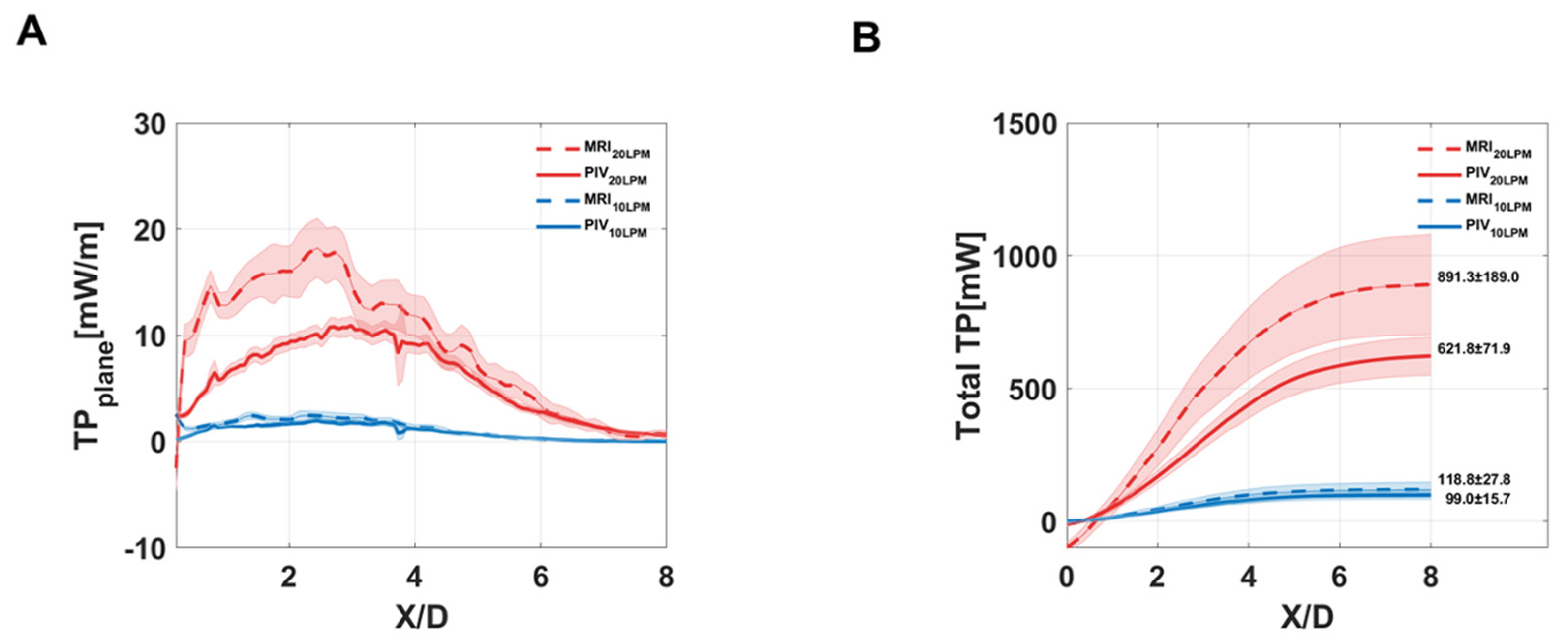
While the 4D flow MRI showed its potential to visualize all elements of RST, an erroneous RST values were also observed near the stenosis. This could induce spurious negative TP at the stenotic region. Unlike positive TP, which indicates energy transfer from the mean flow to the fluctuating velocity, negative TP is a rarely observable phenomenon because it indicates energy backscattering from the fluctuating velocity to the mean flow [16,21,22]. Therefore, it is likely that most of the negative TP values associated with stenotic flow stem from incorrect measurements in the off-diagonal elements. To minimize the measurement error, previous studies have employed the multi-Venc approach to obtain the best estimates possible and filter negative TP for quantification [16,23]. A recent study used another approach and filtered only the negative diagonal components of Reynolds stress since the diagonal terms cannot be negative by definition [24].

Despite the differences in absolute magnitude of turbulence parameters, the 4D flow MRI turbulence quantification is linearly correlated to the ground-truth PIV measurements. It is expected that the further extended method would fill this gap between the methods, however, the current 4D flow MRI turbulence estimation would be better understood as relative quantification showing how a high level of turbulence developed in the flow. Utilizing the 4D flow MRI turbulence quantification for validations of experimental measurements or CFD turbulence models should be avoided.

Despite the experimental flow is not exactly the same as the human blood flow, the flow rate of 20 L/min and the peak velocity of 1–2 m/s presented in this study are close to the normal aortic flow [2]. However, it should be also noted that MRI measurement accuracy might be affected beyond the tested condition.

The discrepancy of turbulent parameters from MRI and PIV can be from both measurements. MRI turbulence mapping can be affected by the flow displacement artifact, high-order terms, and assumption of Gaussian intravoxel velocity distribution [10]. The current limitation of MRI turbulence measurement can be improved as the better gradient system of MRI and better intravoxel velocity model are developed. On the other hand, PIV measurement can be also affected by the interrogation window size and particle density. As the PIV uses the statistical average velocity within the interrogation window, it can be a reason for the underestimation of turbulence parameters [25].

In this study, we validated the 4D flow MRI velocity and turbulence measurements. As the velocity measurements from the 4D flow MRI and PIV were qualitatively well agreed, it indicates 4D flow MRI can measure the turbulent blood flow in clinics. Despite the discrepancy with PIV, it is also shown that 4D flow MRI can measure turbulent parameters such as the Reynolds stress. This indicates that 4D flow MRI can be usefully used to assess the turbulent flow in the patients with valvular diseases such as aortic stenosis

The limitations of this study are the lack of pulsatile flow experiments and the limited geometry for the test. Depending on the geometry of the flow conduit, turbulence parameters can be affected. The turbulence in the pulsatile flow was not compared with PIV because of the experimental difficulties. However, the use of a steady flow reduced the complexity of the study, facilitating the examination of other desired parameters. The results presented in this paper were all obtained using a static flow phantom. Therefore, the effects of motion and gating issues during the scanning of in-vivo subjects remain to be investigated.